CrusaderFrank
Diamond Member
- May 20, 2009
- 163,597
- 90,190
- 2,645
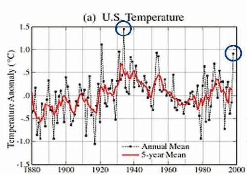
Son of a gun! After the unwarranted "Baseline Adjustment" it's warming all over again!
Follow along with the video below to see how to install our site as a web app on your home screen.
Note: This feature may not be available in some browsers.
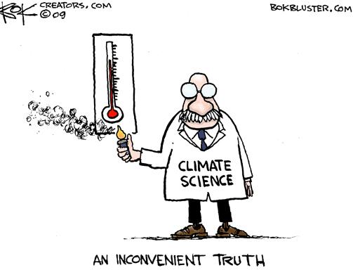
It is all FUDGE, all of it.
The only actual warming in the data is from the growth of urban areas on the surface of the urban area. There is no other actual warming in the data...
NO WARMING in the ATMOSPHERE
NO WARMING in the OCEANS
NO ONGOING NET ICE MELT
NO BREAKOUT in CANE ACTIVITY
NO OCEAN RISE
NO INCREASE in SURFACE AIR PRESSURE
= PLANET EARTH is NOT WARMING
No Warming? No problem!
They just alter the data to fit their false theory
There are some cases in which the correct action at a particular time would have prevented the spread of the fires. However, once a fire gets going in a wind above 30 miles an hour, and most of the really big fires recorded winds of 50+ mph, there is no way of stopping the fire. And the high winds are also knocking down power lines that start fires where there is no easy access. Of course, one could underground the power in the vulnerable areas, and double the cost of electricity, no one would complain about that, right? Big wildfires are going to be a fact of life as a changing climate creates optimum conditions for them. And we simply do not have the resources to eliminate that threat.You shouldn't be criticizing what you obviously don't understand, Debbie.
There were a number of preventative course of actions that could have minimized
the disasters.
Now there are some people that live in an alternative universe, and others that are just to ******* stupid to see what is going on around them.Hide the Decline...
everyone with a brain understood what that meant, that fudging data was casual routine normalcy at climate fraud central...
The key is to clean out the dead fall, which you moronic "environmentalists" prevent at every opportunity.There are some cases in which the correct action at a particular time would have prevented the spread of the fires. However, once a fire gets going in a wind above 30 miles an hour, and most of the really big fires recorded winds of 50+ mph, there is no way of stopping the fire. And the high winds are also knocking down power lines that start fires where there is no easy access. Of course, one could underground the power in the vulnerable areas, and double the cost of electricity, no one would complain about that, right? Big wildfires are going to be a fact of life as a changing climate creates optimum conditions for them. And we simply do not have the resources to eliminate that threat.
Well now, that was from 1858, here is a summary from 2021;The fact is that AT MOST 120PPM of CO2 will raise temperature .0024F

Delta between common air and 100% CO2
Experiment 1: 90-90 = 0
Experiment 2: 100-94 = 6
Experiment 3: 110-99= 11
Experiment 4: 120-100= 20
The incremental heat from 120PPM CO2 is therefore:
Experiment 1: 0
Experiment 2: .00072F
Experiment 3: .00132F
Experiment 4: .0024F


You truly are that ******* dumb. Apparently you have no idea of the size of the forests in the Western US. Or the kind of terrain that those forest are on. And you claim to by a PhD geologist. LOLThe key is to clean out the dead fall, which you moronic "environmentalists" prevent at every opportunity.
Nah, I have no idea having worked as a Hot Shot during my college days.You truly are that ******* dumb. Apparently you have no idea of the size of the forests in the Western US. Or the kind of terrain that those forest are on. And you claim to by a PhD geologist. LOL
Tens of thousands of people are losing their home insurance due to increasing risk of fire and storms. Areas that used to be insurable are no longer insurable or only insurable at a rate that makes the mortgage unaffordable for most. But the deniers still insist nothing is happening. LOL

The article posted was from a laboratory experiment.Well now, that was from 1858, here is a summary from 2021;
Plain Language Summary
Increasing CO2 reduces the rate at which energy leaves Earth, causing a net energy gain at its surface. The resulting warming increases the rate that energy leaves the planet. The planet stops warming once it regains balance. Studies usually assume that doubling atmospheric CO2 always produces the same eventual global temperature rise (called the “equilibrium climate sensitivity”), whatever the starting CO2 level. We show, on the contrary, that in nearly all the computer climate models we have examined, the extra warming for each doubling goes up as the CO2 level increases. In most models, the warmer the climate becomes, the more it has to warm in order to balance a further CO2 doubling because warming becomes less effective at rebalancing the flow of energy. This effect increases projections of warming, especially for scenarios of greatest CO2 increase.
And then the math;
2 Equilibrium Warming
Let T be the globally averaged surface temperature and ΔT ≡ T − T<em>pi</em> be the warming relative to the preindustrial period. We define ΔT<em>eq</em>(C) as the equilibrium warming caused by changing the CO2 concentration from its preindustrial value (pCO2,<em>pi</em> ≈ 280ppm) to a new value (pCO2), where Cis the number of CO2 doublings relative to this preindustrial period,
(1)
Under preindustrial conditions, C<em>pi</em> = 0; in an abrupt 2 × CO2 simulation, C = 1; and so forth. Table S1 is a glossary of all symbols used in this paper.
One condition for equilibrium is that the net top-of-atmosphere radiative flux N (downwards positive) is zero, on average. If we assume that N depends solely on C and T, then we can express a change in N in an abrupt n × CO2 simulation as an initial change due to C and a subsequent change due to T:
(2)
(3)
(4)
F is the radiative forcing, the change in N relative to a given initial condition (C<em>i</em>, T<em>i</em>) caused by C doublings of CO2 while holding surface temperature fixed (F(C<em>i</em>, T<em>i</em>, C) ≡ N(C<em>i</em> + C, T<em>i</em>) − N(C<em>i</em>, T<em>i</em>)), and λ is the radiative feedback, the dependence of N on T (λ(C, T) ≡ ∂N(C, T)/∂T), where the sign convention implies the feedback is typically negative. We can find ΔT<em>eq</em>(C) by setting N(C, T) = 0:
(5)
where we assume N(C<em>pi</em>, T<em>pi</em>) = 0, since the preindustrial climate was roughly in equilibrium.
Under preindustrial concentrations, the spectral line shape of CO2 absorption bands creates a logarithmic dependence of N on changes in pCO2, so that the forcing per CO2doubling () is often assumed to be constant (Myhre et al., 1998). Our definition of radiative forcing also includes adjustments of the atmosphere, land, and ocean to CO2 changes that occur independently of subsequent changes in surface temperature (e.g., Kamae et al., 2015; Sherwood et al., 2014). This “effective radiative forcing” is also often assumed to be constant per CO2 doubling (Forster et al., 2016), as is the radiative feedback (Gregory et al., 2004; Hansen et al., 1985). Substituting these constant terms into Equation 5, we can solve for ΔT<em>eq</em>(C):
(6)
Assuming a constantand λ is equivalent to approximating N(T, C) with the linear Taylor expansion of N around preindustrial values of C<em>pi</em> and T<em>pi</em> (i.e.,, where C = ΔC because C<em>pi</em> = 0). The linear approximation of Equation 6 is ubiquitous in climate science (e.g., Knutti et al., 2017; Stocker et al., 2013).
The linear approximation implies that the equilibrium climate sensitivity (ΔT2<em>x</em>), the equilibrium warming per CO2 doubling, is simply, which, being a ratio of two constants, is itself a constant. It should therefore not matter how many CO2 doublings are used to estimate it since ΔT2<em>x</em> = ΔT<em>eq</em> (C1)/C1 = ΔT<em>eq</em> (C2)/C2. Figure 1a shows instead that our estimates of ΔT<em>eq</em>(C)/C increase with CO2 concentration for 13 of 14 models. Colored bars show estimates made by extrapolating regressions of years 21–150 of N against ΔT to equilibrium (N = 0) for abrupt 2<em>C</em> × CO2 simulations (Gregory et al., 2004, see also solid gray lines in Figure S1). In these estimates, N and ΔT are anomalies: for LongRunMIP, we subtract the model's control simulation's mean value; for CMIP6, we subtract the linear fit of the control simulation after the branch point for the abrupt n × CO2 simulations. We use only one ensemble member for each simulation.
Now that is an American Geophysical Union publication, and I am sure that old Westie thinks he is smarter than all the real scientists in the AGU.
Well now, that was from 1858, here is a summary from 2021;
Plain Language Summary
Increasing CO2 reduces the rate at which energy leaves Earth, causing a net energy gain at its surface. The resulting warming increases the rate that energy leaves the planet. The planet stops warming once it regains balance. Studies usually assume that doubling atmospheric CO2 always produces the same eventual global temperature rise (called the “equilibrium climate sensitivity”), whatever the starting CO2 level. We show, on the contrary, that in nearly all the computer climate models we have examined, the extra warming for each doubling goes up as the CO2 level increases. In most models, the warmer the climate becomes, the more it has to warm in order to balance a further CO2 doubling because warming becomes less effective at rebalancing the flow of energy. This effect increases projections of warming, especially for scenarios of greatest CO2 increase.
And then the math;
2 Equilibrium Warming
Let T be the globally averaged surface temperature and ΔT ≡ T − T<em>pi</em> be the warming relative to the preindustrial period. We define ΔT<em>eq</em>(C) as the equilibrium warming caused by changing the CO2 concentration from its preindustrial value (pCO2,<em>pi</em> ≈ 280ppm) to a new value (pCO2), where Cis the number of CO2 doublings relative to this preindustrial period,
(1)
Under preindustrial conditions, C<em>pi</em> = 0; in an abrupt 2 × CO2 simulation, C = 1; and so forth. Table S1 is a glossary of all symbols used in this paper.
One condition for equilibrium is that the net top-of-atmosphere radiative flux N (downwards positive) is zero, on average. If we assume that N depends solely on C and T, then we can express a change in N in an abrupt n × CO2 simulation as an initial change due to C and a subsequent change due to T:
(2)
(3)
(4)
F is the radiative forcing, the change in N relative to a given initial condition (C<em>i</em>, T<em>i</em>) caused by C doublings of CO2 while holding surface temperature fixed (F(C<em>i</em>, T<em>i</em>, C) ≡ N(C<em>i</em> + C, T<em>i</em>) − N(C<em>i</em>, T<em>i</em>)), and λ is the radiative feedback, the dependence of N on T (λ(C, T) ≡ ∂N(C, T)/∂T), where the sign convention implies the feedback is typically negative. We can find ΔT<em>eq</em>(C) by setting N(C, T) = 0:
(5)
where we assume N(C<em>pi</em>, T<em>pi</em>) = 0, since the preindustrial climate was roughly in equilibrium.
Under preindustrial concentrations, the spectral line shape of CO2 absorption bands creates a logarithmic dependence of N on changes in pCO2, so that the forcing per CO2doubling () is often assumed to be constant (Myhre et al., 1998). Our definition of radiative forcing also includes adjustments of the atmosphere, land, and ocean to CO2 changes that occur independently of subsequent changes in surface temperature (e.g., Kamae et al., 2015; Sherwood et al., 2014). This “effective radiative forcing” is also often assumed to be constant per CO2 doubling (Forster et al., 2016), as is the radiative feedback (Gregory et al., 2004; Hansen et al., 1985). Substituting these constant terms into Equation 5, we can solve for ΔT<em>eq</em>(C):
(6)
Assuming a constantand λ is equivalent to approximating N(T, C) with the linear Taylor expansion of N around preindustrial values of C<em>pi</em> and T<em>pi</em> (i.e.,, where C = ΔC because C<em>pi</em> = 0). The linear approximation of Equation 6 is ubiquitous in climate science (e.g., Knutti et al., 2017; Stocker et al., 2013).
The linear approximation implies that the equilibrium climate sensitivity (ΔT2<em>x</em>), the equilibrium warming per CO2 doubling, is simply, which, being a ratio of two constants, is itself a constant. It should therefore not matter how many CO2 doublings are used to estimate it since ΔT2<em>x</em> = ΔT<em>eq</em> (C1)/C1 = ΔT<em>eq</em> (C2)/C2. Figure 1a shows instead that our estimates of ΔT<em>eq</em>(C)/C increase with CO2 concentration for 13 of 14 models. Colored bars show estimates made by extrapolating regressions of years 21–150 of N against ΔT to equilibrium (N = 0) for abrupt 2<em>C</em> × CO2 simulations (Gregory et al., 2004, see also solid gray lines in Figure S1). In these estimates, N and ΔT are anomalies: for LongRunMIP, we subtract the model's control simulation's mean value; for CMIP6, we subtract the linear fit of the control simulation after the branch point for the abrupt n × CO2 simulations. We use only one ensemble member for each simulation.
Now that is a American Geophysical Union publication, and I am sure that old Westie thinks he is smarter than all the real scientists in the AGU.
Now there are some people that live in an alternative universe, and others that are just to ******* stupid to see what is going on around them.
Well now, that was from 1858, here is a summary from 2021;
Plain Language Summary
Increasing CO2 reduces the rate at which energy leaves Earth, causing a net energy gain at its surface. The resulting warming increases the rate that energy leaves the planet. The planet stops warming once it regains balance. Studies usually assume that doubling atmospheric CO2 always produces the same eventual global temperature rise (called the “equilibrium climate sensitivity”), whatever the starting CO2 level. We show, on the contrary, that in nearly all the computer climate models we have examined, the extra warming for each doubling goes up as the CO2 level increases. In most models, the warmer the climate becomes, the more it has to warm in order to balance a further CO2 doubling because warming becomes less effective at rebalancing the flow of energy. This effect increases projections of warming, especially for scenarios of greatest CO2 increase.
And then the math;
2 Equilibrium Warming
Let T be the globally averaged surface temperature and ΔT ≡ T − T<em>pi</em> be the warming relative to the preindustrial period. We define ΔT<em>eq</em>(C) as the equilibrium warming caused by changing the CO2 concentration from its preindustrial value (pCO2,<em>pi</em> ≈ 280ppm) to a new value (pCO2), where Cis the number of CO2 doublings relative to this preindustrial period,
(1)
Under preindustrial conditions, C<em>pi</em> = 0; in an abrupt 2 × CO2 simulation, C = 1; and so forth. Table S1 is a glossary of all symbols used in this paper.
One condition for equilibrium is that the net top-of-atmosphere radiative flux N (downwards positive) is zero, on average. If we assume that N depends solely on C and T, then we can express a change in N in an abrupt n × CO2 simulation as an initial change due to C and a subsequent change due to T:
(2)
(3)
(4)
F is the radiative forcing, the change in N relative to a given initial condition (C<em>i</em>, T<em>i</em>) caused by C doublings of CO2 while holding surface temperature fixed (F(C<em>i</em>, T<em>i</em>, C) ≡ N(C<em>i</em> + C, T<em>i</em>) − N(C<em>i</em>, T<em>i</em>)), and λ is the radiative feedback, the dependence of N on T (λ(C, T) ≡ ∂N(C, T)/∂T), where the sign convention implies the feedback is typically negative. We can find ΔT<em>eq</em>(C) by setting N(C, T) = 0:
(5)
where we assume N(C<em>pi</em>, T<em>pi</em>) = 0, since the preindustrial climate was roughly in equilibrium.
Under preindustrial concentrations, the spectral line shape of CO2 absorption bands creates a logarithmic dependence of N on changes in pCO2, so that the forcing per CO2doubling () is often assumed to be constant (Myhre et al., 1998). Our definition of radiative forcing also includes adjustments of the atmosphere, land, and ocean to CO2 changes that occur independently of subsequent changes in surface temperature (e.g., Kamae et al., 2015; Sherwood et al., 2014). This “effective radiative forcing” is also often assumed to be constant per CO2 doubling (Forster et al., 2016), as is the radiative feedback (Gregory et al., 2004; Hansen et al., 1985). Substituting these constant terms into Equation 5, we can solve for ΔT<em>eq</em>(C):
(6)
Assuming a constantand λ is equivalent to approximating N(T, C) with the linear Taylor expansion of N around preindustrial values of C<em>pi</em> and T<em>pi</em> (i.e.,, where C = ΔC because C<em>pi</em> = 0). The linear approximation of Equation 6 is ubiquitous in climate science (e.g., Knutti et al., 2017; Stocker et al., 2013).
The linear approximation implies that the equilibrium climate sensitivity (ΔT2<em>x</em>), the equilibrium warming per CO2 doubling, is simply, which, being a ratio of two constants, is itself a constant. It should therefore not matter how many CO2 doublings are used to estimate it since ΔT2<em>x</em> = ΔT<em>eq</em> (C1)/C1 = ΔT<em>eq</em> (C2)/C2. Figure 1a shows instead that our estimates of ΔT<em>eq</em>(C)/C increase with CO2 concentration for 13 of 14 models. Colored bars show estimates made by extrapolating regressions of years 21–150 of N against ΔT to equilibrium (N = 0) for abrupt 2<em>C</em> × CO2 simulations (Gregory et al., 2004, see also solid gray lines in Figure S1). In these estimates, N and ΔT are anomalies: for LongRunMIP, we subtract the model's control simulation's mean value; for CMIP6, we subtract the linear fit of the control simulation after the branch point for the abrupt n × CO2 simulations. We use only one ensemble member for each simulation.
Now that is a American Geophysical Union publication, and I am sure that old Westie thinks he is smarter than all the real scientists in the AGU.

 www.nbcnews.com
Climate alarmists falsely claim the world is literally on fire
In 2022, the last year for which there are complete data, the world hit a record low of 2.2% burned area.nypost.com
As the articles states, wild fire burnt area is less and no one is reporting it.
The reason why no one is reporting it, is because if doesn't follow the narrative, the political science. Everyone is on the band wagon to charge everyone more and more, and the excuse to do so is climate change. The city I used to live in is built on a flood plain.Historical notes shows the city has experienced floods for hundreds of years, but the floods from 2000 are classed as the result of man made climate change. We live in stupid times.
The Weather and climate in Southern Scotland is improving!!
Indeed, the idiocy required to believe CO2 FRAUD is breathtaking.
Your side has ZERO actual evidence.
Surface Air Pressure prove
1. Earth is NOT WARMING
2. Earth is not experiencing an ongoing net ice melt
and maybe that is why
Bill Gates defunded his climate activist group
Blackrock divested from climate stocks
There has not yet been a Million MORON March on DC protesting "climate denialism"
Sure, and I am Napoleon reincarnated. LOL And just where are you going to get the manpower to clear all the debris in the forests? There are 294,275 square miles of forest in the US. That is 818,814,000 acres. And much of the terrain is rather rough. How many tens of thousands of people are you going to hire on a year round basis for that work? Where are you going to get them, and how are you going to pay for them. Westie, you are an unfunny joke.Nah, I have no idea having worked as a Hot Shot during my college days.
You truly are a ignorant ****. Deadfall clearance is a year round job. Except your environutjobs refuse to allow it to be done.
You all are nothing but mental midgets
Another really dumb **** post.Arctic Ice free? Check
Antarctica Ice Sheet melting, massive Ice Loss? Check
Sea Levels rise? CheckView attachment 1132216View attachment 1132218

 earthobservatory.nasa.gov