It took 12 million years for the temperature to finally respond to CO2

[ding]

No it doesn't. It indicates that you are an idiot for questioning data that is widely accepted and readily available from multiple sources. Clearly you are concerned with what the data proves that you would try to discredit it.

Stop lying. You do not have data from multiple sources. You have data from one single source, which appears to be faked (being you won't show the source, and that the paper it claims to be from doesn't show such data), and you actively refuse to look at any other data.

In contrast, I posted what the data from multiple sources says, in Royer (2006), which summarizes all the other studies. The data from multiple sources flatly contradict your claims, being that no CO2 spike is shown. By your own standards, you are totally wrong because multiple sources say so.

http://droyer.web.wesleyan.edu/PhanCO2(GCA).pdf

Do you have the courage to address this, Ding? After all, over in the religion folder, you just bragged about how your religion gives you courage. Funny, how there's no sign of any courage from you over here. Instead, we just see you running away, over and over.

“Around half of the CO2 available at the time,” Bujak said . “Levels dropped from between 2500 and 3500 [parts per million] to between 1500 and 1600 ppm.”*44

The fern that changed the world

 

[ding]

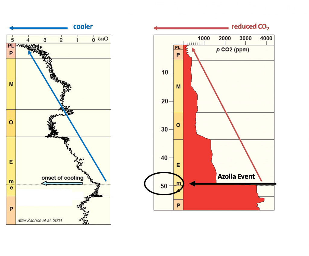
FIGURE 2. Evolution of atmospheric CO2 levels and global climate over the past 65 million years.
From the following article:
An early Cenozoic perspective on greenhouse warming and carbon-cycle dynamics

James C. Zachos, Gerald R. Dickens & Richard E. Zeebe

Nature 451, 279-283(17 January 2008)

doi:10.1038/nature06588

back to article

a, Cenozoic pCO2 for the period 0 to 65 million years ago. Data are a compilation of marine (see ref. 5 for original sources) and lacustrine24 proxy records. The dashed horizontal line represents the maximum pCO2 for the Neogene (Miocene to present) and the minimum pCO2 for the early Eocene (1,125 p.p.m.v.), as constrained by calculations of equilibrium with Na–CO3 mineral phases (vertical bars, where the length of the bars indicates the range of pCO2 over which the mineral phases are stable) that are found in Neogene and early Eocene lacustrine deposits24. The vertical distance between the upper and lower coloured lines shows the range of uncertainty for the alkenone and boron proxies. b, The climate for the same period (0 to 65 million years ago). The climate curve is a stacked deep-sea benthic foraminiferal oxygen-isotope curve based on records from Deep Sea Drilling Project and Ocean Drilling Program sites6, updated with high-resolution records for the interval spanning the middle Eocene to the middle Miocene25, 26, 27. Because the temporal and spatial distribution of records used in the stack are uneven, resulting in some biasing, the raw data were smoothed by using a five-point running mean. The

18O temperature scale, on the right axis, was computed on the assumption of an ice-free ocean; it therefore applies only to the time preceding the onset of large-scale glaciation on Antarctica (about 35 million years ago). The figure clearly shows the 2-million-year-long Early Eocene Climatic Optimum and the more transient Mid-Eocene Climatic Optimum, and the very short-lived early Eocene hyperthermals such as the PETM (also known as Eocene Thermal Maximum 1, ETM1) and Eocene Thermal Maximum 2 (ETM2; also known as ELMO).

, parts per thousand.

Figure 2 : An early Cenozoic perspective on greenhouse warming and carbon-cycle dynamics : Nature

From my perspective, very interesting graphs. You see, during the Miocene, the temperature was pretty stable. As was the CO2 levels. But, as the Isthmus of Panama closed, you see that plunge in temperatures, and the glaciation cycles of the Northern Hemisphere. So, the combination of the closing of the Isthmus and the low CO2 levels resulted in our present ice age cycles. Since we have never seen a spike of GHGs like that we are creating with the combination of the closed Isthmus and a north polar ice cap, kind of hard to predict exactly what is going to happen. By what we are already observing in the Arctic and Greenland, we will see some major changes there by 2030.

You are proving my point. Look at the data.

 

[ding]

Figure F6. Cenozoic pCO2 as estimated by the B isotope method (Pearson and Palmer, 2000) and by alkenone carbon isotope method (Pagani et al., 1999).

 

[Old Rocks]

The early part of the Cenozoic therefore inherited the Mesozoic greenhouse world, which continued through the Paleocene. Extensive volcanism associated with the Greenland mantle plume injected enormous quantities of gases, including carbon dioxide, into the atmosphere, raising temperatures and triggering the release of methane clathrates. This potent combination resulted in high levels of greenhouse gases 55 million years ago during the Paleocene-Eocene Thermal Maximum (PETM, aka. the Early Eocene Thermal Maximum, EETM).

The Geological Society of London - The Arctic Azolla event

So, what they are saying here is that the injection of GHGs created the very rapid heat up of the PETM.

 

[ding]

The early part of the Cenozoic therefore inherited the Mesozoic greenhouse world, which continued through the Paleocene. Extensive volcanism associated with the Greenland mantle plume injected enormous quantities of gases, including carbon dioxide, into the atmosphere, raising temperatures and triggering the release of methane clathrates. This potent combination resulted in high levels of greenhouse gases 55 million years ago during the Paleocene-Eocene Thermal Maximum (PETM, aka. the Early Eocene Thermal Maximum, EETM).

The Geological Society of London - The Arctic Azolla event

So, what they are saying here is that the injection of GHGs created the very rapid heat up of the PETM.

"...Calculations of Azolla’s volume during the event show that it had a huge impact on the world’s climate. The billions of tiny plants drew down the carbon dioxide needed for their growth directly from the atmosphere, reducing greenhouse gases, and ending the greenhouse climate that had prevailed for hundreds of millions of years. Levels of atmospheric carbon dioxide that had been as high as 2500 to 3500ppm before the Azolla Event were reduced by up to a half by the Azolla Event.

Atmospheric carbon dioxide continued to fall over the next 49 million years due to mountain uplift and changing oceanic currents that sequestered even more carbon dioxide. As atmospheric carbon dioxide fell below 1000ppm about 40 million years ago, permanent ice and snow increased in Antarctica. Then, as it fell even lower to 600ppm just 2.6 million years ago, widespread glaciation began in the Arctic, initiating the succession of glacial-interglacial cycles that characterise today’s icehouse world. Present values are just above 400ppm, having risen from pre-industrial values in the mid 18th Century of about 280ppm...."

 

[ding]

 

[Old Rocks]

Calculations of Azolla’s volume during the event show that it had a huge impact on the world’s climate. The billions of tiny plants drew down the carbon dioxide needed for their growth directly from the atmosphere, reducing greenhouse gases, and ending the greenhouse climate that had prevailed for hundreds of millions of years. Levels of atmospheric carbon dioxide that had been as high as 2500 to 3500ppm before the Azolla Event were reduced by up to a half by the Azolla Event.

Atmospheric carbon dioxide continued to fall over the next 49 million years due to mountain uplift and changing oceanic currents that sequestered even more carbon dioxide. As atmospheric carbon dioxide fell below 1000ppm about 40 million years ago, permanent ice and snow increased in Antarctica. Then, as it fell even lower to 600ppm just 2.6 million years ago, widespread glaciation began in the Arctic, initiating the succession of glacial-interglacial cycles that characterise today’s icehouse world. Present values are just above 400ppm, having risen from pre-industrial values in the mid 18th Century of about 280ppm.

The Geological Society of London - The Arctic Azolla event

So the Arctic began to ice over as we dipped below 600 ppm. And we are at 400+ ppm and rapidly rising.

Seems to me that one of the points that paper makes is that GHGs are one of the primary factors influencing the climate.

 

[Old Rocks]

PERFECT STORM
We humans are threatened by a perfect storm as our population passes seven billion thanks to shortages of land, food and energy. Increased emissions of greenhouse gases are also reversing climatic changes that occurred over millions of years. The greenhouse-to-icehouse shift was caused by a succession of processes that took 49 million years, but mankind’s emission of greenhouse gases could reverse this process in just a few decades, changing the climate back to a greenhouse world with dizzying speed. Could Azolla help us combat man-made climate change and also provide local renewable food, livestock feed, biofertilizer and biofuel?

The Geological Society of London - The Arctic Azolla event

So, the authors seem to be making a point exactly opposite of your point. And the onset of Arctic ice was at 600 ppm about 2 million years ago, and we are less than 200 ppm from reversing that level, and at the present rate of increase of atmospheric CO2 and CH4, we will blow past 600 ppm somewhere between 2050 and 2100. In fact, we may well do that before 2050.

 

[ding]

So the Arctic began to ice over as we dipped below 600 ppm. And we are at 400+ ppm and rapidly rising.

Seems to me that one of the points that paper makes is that GHGs are one of the primary factors influencing the climate.

But my point is that it took 12 million years for the temperature to drop after a massive CO2 drawdown.

 

[ding]

PERFECT STORM
We humans are threatened by a perfect storm as our population passes seven billion thanks to shortages of land, food and energy. Increased emissions of greenhouse gases are also reversing climatic changes that occurred over millions of years. The greenhouse-to-icehouse shift was caused by a succession of processes that took 49 million years, but mankind’s emission of greenhouse gases could reverse this process in just a few decades, changing the climate back to a greenhouse world with dizzying speed. Could Azolla help us combat man-made climate change and also provide local renewable food, livestock feed, biofertilizer and biofuel?

The Geological Society of London - The Arctic Azolla event

So, the authors seem to be making a point exactly opposite of your point. And the onset of Arctic ice was at 600 ppm about 2 million years ago, and we are less than 200 ppm from reversing that level, and at the present rate of increase of atmospheric CO2 and CH4, we will blow past 600 ppm somewhere between 2050 and 2100. In fact, we may well do that before 2050.

But my point is that it took 12 million years for the temperature to drop after a massive CO2 drawdown.

 

[Old Rocks]

Well now, if you believe that was truly the case, and there were not other factors involved, then seeing that the temperature is ramping up as we increase the GHGs in the atmosphere, and that it did the same in the PETM and the PT, then I would think that you would be the first to advocate immediate cessation of dumping more GHGs into the atmosphere. After all, if after the warm up, it takes that long to cool, we are condemning tens of coming generations to a much different world than we have known.

 

[ding]

Well now, if you believe that was truly the case, and there were not other factors involved, then seeing that the temperature is ramping up as we increase the GHGs in the atmosphere, and that it did the same in the PETM and the PT, then I would think that you would be the first to advocate immediate cessation of dumping more GHGs into the atmosphere. After all, if after the warm up, it takes that long to cool, we are condemning tens of coming generations to a much different world than we have known.

12 million years. 12 million years.

 

[Old Rocks]

Well now, I don't think that we are going to go up to 3500 ppm. Maybe only 1000 ppm. So, probably be only about a million years. Maybe less. Ain't that just wonderful?

 

[Kosh]

Then what do you believe is driving the current temperature change?

More AGW cult cheery picked data not based in reality!

 

[Old Rocks]

Now Kosh, we have been patiently trying to drive into your single brain cell that it is not the absolute temperature, but the rate of change, that is the problem. And all that implies for agriculture and sea level.