clock precision not limited by the Second Law

[scruffy]

This is thick stuff. But pretty amazing.

The traditional view of clocks as time measurement devices depends on the Second Law of Thermodynamics. Known physical processes are time reversible, and it is only the dissipation predicted by the Second Law that drives the arrow of time forward. In the limit, what the clock is actually measuring is entropy.

https://www.tandfonline.com/doi/full/10.1080/00107514.2020.1837471#abstract

However here is clock that doesn't depend on the Second Law.

Precision is not limited by the second law of thermodynamics - Nature Physics

Clock precision is thought to be fundamentally limited by entropy production in out-of-equilibrium systems. A theoretical work now introduces a quantum clock design where precision grows exponentially with dissipation.

www.nature.com

It uses a quantum spin chain and a single jump process. It is statistical in nature - what the clock is actually measuring is the ticks to a bit error.

"Ticks" in this case, are revolutions around the spin chain. There is coherent transport around the chain, followed by a single dissipative link.

 

[scruffy]

Believe it or not, we actually know very little about probability.

Most of what we know is based on "frequentist" assumptions, where everything is objective, and the empirical has to equal the objective otherwise the assumptions break down.

For instance the probability "distribution" never varies, it's cast in stone. This is why the "all possible paths" construction works, and why the Fisher information metric gives us the amount of information conveyed by a new observation.

Information theory is this way too, the probability has to be a known function for it to work.

But quite obviously, brains don't work this way, the probabilities are almost never known in advance. Brains use an entirely different method called "Bayesian", which is inherently subjective. You're allowed to make guesses about the probabilities, and then adjust those guesses based on observations.

So imagine if you will, a Bayesian version of information theory. Let's say you have a bit transmitted on a wire. Information theory says the bit can be either a 0 or a 1. So you can calculate the uncertainty as - p log p, which means the bit tells you nothing if it's always a 0 or a 1. The only time you get information is if the probability of the bit is "either" a 0 or a 1. In that case the arrival of the bit (the "outcome") is exactly like a coin flip, and information theory says you get 1 bit of information, because you now "know" the outcome.

The coin flip is called a "Bernoulli trial", and depending on the probability of success this is how much information you get:

For this to work, the relationship between the probability and the information must be known in advance, in this case it's a binomial distribution. If you have repeated coin flips you can calculate probabilities with "n choose k" and so on.

But let's say we didn't know the distribution in advance - which is probably the case in most of nonlinear thermodynamics (eg quantum behavior in free space and time). What do your sensibilities tell you about how much information you'd get from the sudden appearance of a bit?

In a way, this situation can be reformulated in terms of an unknown probability distribution. Maybe instead of a binomial Bernoulli distribution you're looking at an exponential Poisson distribution where bits arrive randomly at a rate r. If you know in advance that you're dealing with an exponential distribution you can calculate the information, but what if you don't know that?

Clearly, the bit tells you "something". You just don't know what it is, because you have no context. The Bayesian method lets you define context. The more bits you see, the more context you have. This is formalized by the "prior" and the "posterior" in Bayesian statistics.

The Central Limit Theorem says that eventually, you will have "enough" context.

To figure out what the bits "mean", you have to relate one but to all the other bits. So this becomes a topological problem in set theory. The only requirement is that the bits be "separable", in other words distinguishable. The "meaning" relates to how many ways you can partition N bits in k dimensions, where k is a "guess". So what your brain does is it tries to optimize k. It tries to find the "maximum likelihood" for k, where k grows with N. This is fundamentally a problem in algebraic topology.

This is why "topological" quantum computing is so important. If your bit happens to be a qubit, it can take on any value between 0 and 1 with a continuous uniform distribution. A continuous uniform distribution is a topological "interval" in one dimension. You can no longer think in terms of discrete probabilities, because the number of points (possible outcomes) in the interval is uncountably infinite. The cardinality of the interval is the same as the cardinality of R. (Georg Cantor proved this, and many other similar topological conceptualizations).

So information theory won't work in this context because the probability of any given point outcome is ZERO. You have to go to the von Neumann formulation which defines what is essentially a "margin of confidence" - it is what the Bayesians call a "credible" interval. Topologically this is equivalent to partitioning the interval. For example you can say "I am 95% sure that the outcome will be between .1 and .9", or some similar statement of confidence. This is equivalent to partitioning the interval into three subsets, where the bulk of the interval is in the middle subset. Therefore information no longer has a defined value, it only has a confidence level - because the cardinality of each subset is the same as the cardinality of the original (total) set.

The astute observer will understand how this relates to the OP.

 

[scruffy]

Oh - here is additional information:

Bayesians represent uncertainty with probabilities.

This means the posterior can be defined as a recursion.

A recursion is how Cantor defined dusts, how Peano defined space filling curves, and how Mandelbrot defined fractals.

In Bayesian statistics, the posterior is defined as the likelihood times the prior.

Where the prior is itself the posterior of a more distant prior. Hence, the recursion.

The base case, is a "guess".

So formally this equates with an iterative regression, against a dataset that is constantly growing. In other words, a stochastic reaction-diffusion equation, which is the same thing we find in nonlinear thermodynamics.

You can imagine optimizing a traveling salesman problem, where the number of cities grows with each iteration. In this case, the initial guess is always 0. (In other words the salesman doesn't have to travel, because there's only one city). But new cities are created at random distances with each iteration. You can use Lyapunov's method to calculate stability based on rate and distance. In some cases you'll get a well behaved cost function and the solution will converge.

 

[scruffy]

Okay, not sure if anyone understands what I'm talking about - but I'm going to coin a phrase.

At least I think I'm coining it, others have surely thought about it before but I can't find it in the literature.

The term is: "continuous recursion".

It has a specific meaning. It is not to be confused with "recursively continuous", which has a different meaning.

Here is a baseline definition:

An ordinary recursion is iterative. That means, it proceeds in discrete steps, which you can count. Even if the recursion is infinite, you can still count the steps (they're "countably infinite"). An example of an infinite recursion is a Cantor Dust. Each subdivision is a step. The steps can be asynchronous for different sub intervals, but they must always occur in order. An ordinary recursion therefore looks like this:

[x] = baseline
while(1)
... [x] = p([x])

The brackets signify that x can be an array, or a set. And, you (or the computer) can count how many times the process p is invoked. It may generate new elements, in which case they get added to the set. The process p proceeds element-wise on all members of x.

For example - in a Cantor Dust the baseline is x = the unit interval [0,1], and the process p says "cut each element into 3 parts". In the first iteration, the initial member of the set is destroyed, because it's cut into 3 parts. However each part is added back into the set, so after 1 iteration x has 3 members. If the recursion is synchronous x grows as 3^n, where n is the number of iterations. We could also do it asynchronously, by assigning available resources from a pool of k processors.

So now, consider this in differential form. We start with something that looks like this in the synchronous case:

x(t+1) = f(x(t))

where f = p (f is used here mainly to relate the discussion to the familiar math of differential equations). This looks very much like an ordinary delay equation. The problem here is we can NOT convert this into simple differential form right away. Ordinarily we would take the limit as dt => 0, but the issue is that x is discontinuous, even in the limit. The instant we apply p we have a step in x (one interval becomes 3).

"If" we have an asynchronous process, we could use a trick that was used by the early physicists, called "time coarse graining", to turn this APPROXIMATELY into an ordinary differential equation for purposes of analysis and thought experimentation, except for the discontinuity in x. We would end up with the world's simplest differential equation, x' = f(x).

But since we have a discontinuous x, we have no choice but to treat x as a random variable and use the Ito or Langevin calculus to make this look like a stochastic differential equation. To do that, we have to make the count of set elements explicit. And, we have to restrict our process p so that only one sub element is updated at a time. In practice then, this becomes a Monte Carlo algorithm where the random variable chooses which set member will be updated next. So this algorithm ends up looking exactly like a Hopfield neural network, except for the discontinuity in x (which in the Hopfield case could be considered as "the number of neurons").

With this knowledge we can now reformulate our algorithm as a genetic equation, where the chosen interval "dies" at each step, and 3 new intervals are "born" in its place. And note that we are NOT using a genetic method to solve the differential equation, we're doing the exact opposite. If we formulate our scenario in terms of population dynamics though, we can once again consider the action of k simultaneous processors, because more than one person can die and be born at the same time.

We still have a problem though. Population is discrete. You can have 20 people, but not 20.1 people. Our number of intervals (count of members in x) has to be discrete. Since we've already used n for the number of iterations and k for the number of processors, let's use m for the number of members in x.

To handle discrete components in stochastic differential equations we have to use a "master equation", which translates the evolution into a "transition matrix". Information on master equations can be found here:

Master equation - Wikipedia

en.wikipedia.org

These master equations are computationally difficult, much more so than ordinary differential equations - although some specific cases can be represented as coupled ODE's. For those who are interested, explanations can be found in these references, in increasing order of complexity:

Mastering the Master Equation

Dive into the world of statistical mechanics with our in-depth guide to the Master Equation, exploring its principles, applications, and significance.

www.numberanalytics.com

http://biotheory.phys.cwru.edu/phys320/phys320_master_equation_I.pdf

https://ifisc.uib-csic.es/raul/CURSOS/SP/Introduction_to_master_equations.pdf

The relevant part of the master equation is the "jump process", which describes our discontinuity.

But now that we understand the landscape, let's return to the point of this post, which is the concept of a continuous recursion. The recursion we just looked at occurs in discrete time (or processing) steps, and the closest we could get to continuity was stipulating "one update at a time" and then summing over updates. So what then, is a "continuous" recursion? A clue comes from the physics of quantum entanglement. Here, we have quantum fluctuations in one body that act as "measurements" on another. Every time a fluctuation occurs some information is transferred from one body to the other, and the net result is a constant exchange of information. Which is, in fact, what keeps the two bodies entangled - their "correlation". Calculating the higher order moments in a quantum many-body scenario is a computational nightmare. However it can be done. Here is an example:

https://link.aps.org/doi/10.1103/PhysRevB.98.205143#:~:text=Abstract,system%20with%20strong%20hyperfine%20interaction.

Our scenario is formally equivalent to "continuous measurement theory" in quantum mechanics.

Here are some tidbits on that:

A Straightforward Introduction to Continuous Quantum Measurement

We present a pedagogical treatment of the formalism of continuous quantum measurement. Our aim is to show the reader how the equations describing such measurements are derived and manipulated in a direct manner. We also give elementary background material for those new to measurement theory, and...

arxiv.org

https://www.sciencedirect.com/science/article/abs/pii/003448779390037F

We can define a continuous recursion as a process p in the "neighborhood"' of an element x.

Quantum Many-Body Dynamics

This Collection highlights theoretical and experimental original research and commissioned commentary on topics in quantum many-body dynamics. The

www.nature.com

Especially check the highlighted section in this link:

The promises and challenges of many-body quantum technologies: A focus on quantum engines - Nature Communications

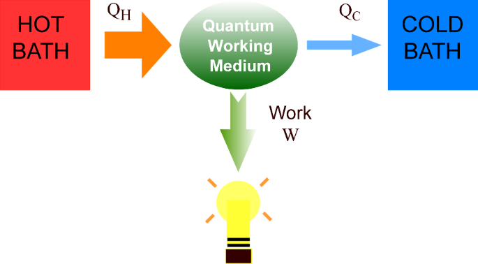
Can many-body systems be beneficial to designing quantum technologies? We address this question by examining quantum engines, where recent studies indicate potential benefits through the harnessing of many-body effects, such as divergences close to phase transitions. However, open questions...

www.nature.com

High precision quantum thermometer is the same as the high precision time definition in the OP.

One can also consider the "process" in terms of fields acting on the elements of x.

Higher order correlations for fluctuations in the presence of fields

The higher order moments of the fluctuations for the thermodynamical systems in the presence of fields are investigated in the framework of a theoretical method. The metod uses a generalized statistical ensemble consonant with the adequate expression for the generalized internal energy. The...

arxiv.org

In the transform domain, we can perform topological recursion on spectra.

Topological recursion - Wikipedia

en.wikipedia.org

https://www.sciencedirect.com/science/article/abs/pii/S0001870823006163

The principle is stated in a different way here:

Topological Recursion

www.math.uni-sb.de

... topological recursion is a recursive formula which computes a family of differential forms associated to a given spectral curve. It turns out these forms admit nice mathematical properties and compute interesting quantities in various field of mathematics. To mention some relations, the topological recursion computes

• Correlations functions in Random Matrix Theory,
• Hurwitz numbers in Enumerative Geometry.
• Gromov-Witten invariants and intersection numbers