Climate Change Threatens Trout

[Star]

.
If you like to fish or if you like to eat fish, climate change is going to change your hobby and your dining.


Hybrid Trout Threaten Montana's Native Cutthroats

by Christopher Joyce
May 27, 2014

Many parts of the U.S. have been getting warmer over the past several decades, and also experiencing persistent drought. Wildlife often can't adjust. Among the species that are struggling is one of the American West's most highly prized fish — the cutthroat trout.

<snip>

The nonnative fish are rainbow trout. They were introduced in Western lakes and streams decades ago to give anglers more fish to catch. The rainbows mostly stayed well down in the valleys, because mountain water at higher elevations — where cutthroat spawn — was too cold, and the amount of water in the streams wasn't right for rainbows.

But over the past few decades, stream flow at higher elevations is down and water temperature is up. These new conditions favor rainbow trout. So rainbows are moving upstream. When they meet the cutthroat, they mate and create a hybrid — essentially, a different type of trout.

<snip>

Now, you might think, so what? Surely a trout's a trout by any other name. But trout fishing brings in tens of millions of dollars (just in Montana), and lots of anglers want to catch native cutthroats — they're as picky about their trout as the trout are about where they spawn.
More important, biologists like Muhlfeld who have been tracking the reproductive success of these hybrids worry that might die out too, leaving fewer fish overall. Recent genetic evidence that he and his colleagues published this week in the journal Nature suggests the hybrid trout aren't doing well at all.

<snip>

.

 

[waltky]

Granny says, "Dat's right - purt soon dey gonna make ever'body wear gas masks whilst dey's trout fishin'...

UN Climate Chief: 'Not Very Far' from Considering 'Climate Change as a Public Health Emergency'
August 28, 2014 – Secretary of State John Kerry has called climate change “the biggest challenge of all that we face right now,” and his French counterpart has warned of climate “chaos” in 500 days, and now the U.N. climate change chief is implying that climate change can be viewed on a par with the deadly Ebola outbreak.

Christiana Figueres told a World Health Organization (WHO)-hosted event in Geneva Wednesday that “we are not very far” from the point where climate change should be declared an international public health emergency, according to her prepared remarks. Addressing a three-day global conference on health and climate – the first of its kind – Figueres said in remarks directed at WHO Director-General Margaret Chan, “Dear Margaret, as much as would like you to, I am fully aware of the fact that you have not convened the international health regulations emergency committee to consider climate change as a public health emergency of international concern.” “However, we are not very far from this,” she added. The committee referred to by Figueres is the expert body on whose advice the WHO three weeks ago declared the Ebola outbreak in West Africa to be a “public health emergency of international concern” (PHEIC).

Under international health regulations, a PHEIC is declared in a case where “an extraordinary event” is determined to constitute a public health risk through the international spread of disease; and “to potentially require a coordinated international response.” In her speech Figueres, who is executive secretary of the U.N. Framework Convention on Climate Change (UNFCCC) said that while it was easy to view climate change as “the equivalent of a disease” it was actually the symptom. “The disease is something we rarely admit,” she said. “The disease is humanity’s unhealthy dependence on fossil fuels, deforestation and land use that depletes natural resources.” “At the heart of an effective response to climate change is the challenge of taking responsibility for our actions and above all, making tough decisions to change the patterns that have been at the base of our development over the past 100 years, if we are to prevent severe worsening of health and quality of life conditions over the next 100 years.”

The U.N. says climate change is having an impact on health in numerous ways, including malnutrition due to crop failures arising from changing weather patterns; water scarcity; the spread of water-borne disease resulting from rising temperatures; and the effect of carbon emissions on rates of cancer and respiratory disease rates. Speaking at the conference Wednesday, Chan linked climate change to the emergence of new human diseases. She said many of these originate in wild animals, whose populations, concentration and incursion into areas where humans live are impacted by climate variables. But she cautioned against speculation that Ebola may be affected by climate. “I am aware of speculation that climate change may influence the frequency of outbreaks of Ebola virus disease,” she said. “I must emphasize we have no evidence that this is the case.”

Paris agreement will be ‘universal and applicable to all countries’

 

[SSDD]

.
If you like to fish or if you like to eat fish, climate change is going to change your hobby and your dining.


Hybrid Trout Threaten Montana's Native Cutthroats

by Christopher Joyce
May 27, 2014

Many parts of the U.S. have been getting warmer over the past several decades, and also experiencing persistent drought. Wildlife often can't adjust. Among the species that are struggling is one of the American West's most highly prized fish — the cutthroat trout.

<snip>

The nonnative fish are rainbow trout. They were introduced in Western lakes and streams decades ago to give anglers more fish to catch. The rainbows mostly stayed well down in the valleys, because mountain water at higher elevations — where cutthroat spawn — was too cold, and the amount of water in the streams wasn't right for rainbows.

But over the past few decades, stream flow at higher elevations is down and water temperature is up. These new conditions favor rainbow trout. So rainbows are moving upstream. When they meet the cutthroat, they mate and create a hybrid — essentially, a different type of trout.

<snip>

Now, you might think, so what? Surely a trout's a trout by any other name. But trout fishing brings in tens of millions of dollars (just in Montana), and lots of anglers want to catch native cutthroats — they're as picky about their trout as the trout are about where they spawn.
More important, biologists like Muhlfeld who have been tracking the reproductive success of these hybrids worry that might die out too, leaving fewer fish overall. Recent genetic evidence that he and his colleagues published this week in the journal Nature suggests the hybrid trout aren't doing well at all.

<snip>

.

The CRN network....a network of triple redundant sensors, so pristinely placed that no correction is necessary says that for the decade it has been in operation the temperature in the US has been in decline...the raw data, what there is of it says that the temperature in the US has been in decline since the 1940's. The US is certainly not getting warmer....just more climate alarmist BS.

 

[Crick]

You admit that most sensors require calibration (ie, adjustment) than freely base your conclusions on uncalibrated data. Swift like rock, smart like tree.

 

[mudwhistle]

Trick or Trout.....

 

[Stephanie]

We're all going DIE we are DOOOMED

run for cover

zzzzzzzzzzz

Do these "chicken little warmers) ever have anything POSITIVE to say?

 

[SSDD]

You admit that most sensors require calibration (ie, adjustment) than freely base your conclusions on uncalibrated data. Swift like rock, smart like tree.

I agree that sensors located in areas near A/C exhaust fans, and on airport runways need to be adjusted down...I haven't really seen any sensors in areas that need to be adjusted up which is what climate science tends to do and I am still waiting for a rational, scientifically sound reason to adjust temperature data taken more than 40 years ago down....and as to the adjustments that are being done...the CRN network has shown at least the past decade of adjustments to be wrong...since adjusted data shows a warming trend while the CRN shows a slight cooling trend.

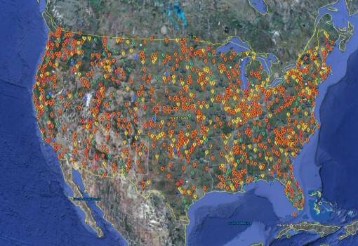
Here is what the state of the USHCN network looks like...explain why temperatures are constantly adjusted up...

 

[Crick]

Why and how adjustments were made to the USHCN data

GHCN Global Gridded Data

The US Historical Climatology Network is a high-quality moderate sized data set of monthly averaged maximum, minimum, and mean temperature and total monthly precipitation developed to assist in the detection of regional climate change. The USHCN is comprised of 1221 high-quality stations from the U.S. Cooperative Observing Network within the 48 contiguous United States. An additional data set containing 46 stations for Alaska is also available; however, data for these stations are not adjusted for inhomogeneities as outlined below for the USHCN. The period of record varies for each station but generally includes the period 1900-1995. The stations were chosen using a number of criteria including length of period of record, percent missing data, number of station moves and other station changes that may affect the data homogeneity, and spatial coverage. Included with the data set are metadata files that contain station history information about station moves, instrumentation, observing times, and elevation.

The USHCN was developed and is maintained at the National Climatic Data Center (NCDC) and the Carbon Dioxide Information and Analysis Center (CDIAC) of Oak Ridge National Laboratory through a cooperative agreement between the NCDC and the U.S. Department of Energy. Currently it is distributed by NCDC and by CDIAC on various computer media including anonymous ftp.

Quality Control, Homogeneity Testing, and Adjustment Procedures
The data for each station in the USHCN are subjected to the following quality control and homogeneity testing and adjustment procedures

1. • A quality control procedure is performed that uses trimmed means and standard deviations in comparison with surrounding stations to identify suspects (> 3.5 standard deviations away from the mean) and outliers (> 5.0 standard deviations). Until recently these suspects and outliers were hand-verified with the original records. However, with the development at the NCDC of more sophisticated QC procedures this has been found to be unnecessary.
   • Next, the temperature data are adjusted for the time-of-observation bias (Karl, et al. 1986) which occurs when observing times are changed from midnight to some time earlier in the day. The TOB is the first of several adjustments. The ending time of the 24 hour climatological day varies from station to station and/or over a period of years at a given station. The TOB introduces a non climatic bias into the monthly means. The TOB software is an empirical model used to estimate the time of observation biases associated with different observation schedules and the routine computes the TOB with respect to daily readings taken at midnight. Details on the procedure are given in, "A Model to Estimate the Time of Observation Bias Associated with Monthly Mean Maximum, Minimum, and Mean Temperatures." by Karl, Williams, et al.1986, Journal of Climate and Applied Meteorology 15: 145-160.
   • Temperature data at stations that have the Maximum/Minimum Temperature System (MMTS) are adjusted for the bias introduced when the liquid-in-glass thermometers were replaced with the MMTS (Quayle, et al. 1991). The TOB debiased data are input into the MMTS program and is the second adjustment. The MMTS program debiases the data obtained from stations with MMTS sensors. The NWS has replaced a majority of the liquid-in-glass thermometers in wooden Cotton-Region shelters with thermistor based maximum-minimum temperature systems (MMTS) housed in smaller plastic shelters. This adjustment removes the MMTS bias for stations so equipped with this type of sensor. The adjustment factors are most appropriate for use when time series of states or larger areas are required. Specific details on the procedures used are given in, "Effects of Recent Thermometer Changes in the Cooperative Network" by Quayle, Easterling, et al. 1991, Bulletin of the American Meteorological Society 72:1718-1724.
   • The homogeneity adjustment scheme described in Karl and Williams (1987) is performed using the station history metadata file to account for time series discontinuities due to random station moves and other station changes. The debiased data from the second adjustment are then entered into the Station History Adjustment Program or SHAP. The SHAP allows a climatological time series of temperature and precipitation adjustment for station inhomogeneities using station history information and is the third adjustment. The adjusted data retains its original scale and is not an anomaly series. The methodology uses the concepts of relative homogeneity and standard parametric (temperature) and non parametric (precipitation) statistics to adjust the data. In addition, this technique provides an estimate of the confidence interval associated with each adjustment. The SHAP program debiases the data with respect to changes other than the MMTS conversion to produced the "adjusted data". Specific details on the procedures used are given in, "An Approach to Adjusting Climatological Time Series for Discontinuous Inhomogeneities" by Karl, and Williams, Jr. 1987, Journal of Climate and Applied Meteorology 26:1744-1763.
   • Estimates for missing data are provided using a procedure similar to that used in the homogeneity adjustment scheme in step three. This fourth adjustment uses the debiased data from the third adjustment (SHAP) and fills in missing original data when needed (i.e. calculates estimated data) based on a "network" of the best correlated nearby stations. The FILNET program also completed the data adjustment process for stations that moved too often for the SHAP program to estimate the adjustments needed to debias the data.
     Each of the above adjustments is done is a sequential manner. The areal edits are preformed first and then the data are passed through the following programs (TOBS, MMTS, SHAP and FILNET). At the end of each program, a dataset is produced and the graphs below show the annual temperature departures for each of the adjusted values.
   • The final adjustment is for an urban warming bias which uses the regression approach outlined in Karl, et al. (1988). The result of this adjustment is the "final" version of the data. Details on the urban warming adjustment are available in "Urbanization: Its Detection and Effect in the United States Climate Record" by Karl. T.R., et al., 1988, Journal of Climate 1:1099-1123.

Currently all data adjustments in the USHCN are based on the use of metadata. However station histories are often incomplete or changes that can cause a time series discontinuity, such as replacing a broken thermometer with one that is calibrated differently, are not routinely entered into station history files. Because of this we are developing another step in the processing that will apply a time series discontinuity adjustment scheme described in Peterson and Easterling (1994) and Easterling and Peterson (1995). This methodology does not use station histories and identifies discontinuities in a station's time series using a homogeneous reference series developed from surrounding stations.

To illustrate the effects of each adjustment scheme, we produced annual time series from each data set using the Climate Analysis System (CAS), a software package developed at NCDC that provides a wide-array of analysis options. Although various grid sizes can be used in the analyis of USHCN data, we determined the optimum grid size to be 2.5 degrees X 3.5 degrees. We calculated all anomalies with respect to the base period 1961-1990 and adjusted the time series to the period 1900 - 1910 to simplify the comparison of the different data sets. The following graphs depict the time series resulting from each USHCN data set.

The adjacent [above] plot shows the annual time series calculated from each of the six USHCN data sets. The USHCN adjustment procedures are applied in stepwise fashion so that the effects from each adjustment have a cumulative effect. The data set containing the final adjustment procedure (urbanization adjustments) also contains all of the previous adjustments. Each series contains data from 1900-1999.

It is much easier to evaluate the effects of each adjustment by plotting stepwise differences between USHCN time series. The effect of each successive adjustment is clearly evident in the adjacent [above] plot that shows the differences in the above time series.

[CONTINUED ON NEXT POST]

 

[Crick]

Applying the Time of Observation adjustment (black line) resulted in approximately a 0.3F warming from the late 1960's to the 1990's. The shift from Cotton Region Shelters to the Maximum/Minimum Thermometer System in the mid-1980's is clearly evident in the difference between the TOBS and the MMTS time series (red line). This adjustment created a small warming in the US annual time series during the mid to late 1980's. Application of the Station History Adjustment Procedure (yellow line) resulted in an average increase in US temperatures, especially from 1950 to 1980. During this time, many sites were relocated from city locations to airports and from roof tops to grassy areas. This often resulted in cooler readings than were observed at the previous sites. When adjustments were applied to correct for these artificial changes, average US temperature anomalies were cooler in the first half of the 20th century and effectively warmed throughout the later half. Filling in missing data (blue line) produced cooler temperatures prior to 1915. Adjustments to account for warming due to the effects of urbanization (purple line) cooled the time series an average of 0.1F throughout the period of record.

The adjacent [above] graph shows how the annual raw (areal edited) mean temperature anomalies compare with the anomalies from the data set containing all adjustments (final). The difference of these two time series is shown below

The cumulative effect of all adjustments is approximately a one-half degree Fahrenheit warming in the annual time series over a 50-year period from the 1940's until the last decade of the century

[TBODY] [/TBODY]

 

[Crick]

Now its your turn. Show us why they should NOT have made those adjustments. Or, at the very least, show us some climate scientists (REAL climate scientists) who think they should not have made those adjustments.